简介
- 留下直观印象:OpenCV有哪些图像和视频处理方法,能实现怎样的功能
- 凡是能应用于图像处理的,就能应用于视频 $\rightarrow$ 一帧帧图片
图片处理
1. 颜色空间转换
cv.cvtColor(input_image, flag),其中flag确定转换类型
对于BGR $\rightarrow$ 灰色转换,我们使用标志cv.COLOR_BGR2GRAY
对于BGR同样 $\rightarrow$ HSV,我们使用标志cv.COLOR_BGR2HSV
# 要获取其他标志,使用如下代码
flags = [i for i in dir(cv) if i.startswith('COLOR_')];
print(flags);
# ['COLOR_BAYER_BG2BGR', 'COLOR_BAYER_BG2BGRA', 'COLOR_BAYER_BG2BGR_EA', ...
cap = cv.VideoCapture(0)
while(1):
    #取每一帧
    _, frame = cap.read()
    # 调用cv.cvtColor将帧的颜色从BGR转化成HSV
    hsv = cv.cvtColor(frame, cv.COLOR_BGR2HSV)
    # 定义HSV中蓝色的上下限值,用于取色
    lower_blue = np.array([50,255,255])
    upper_blue = np.array([70,255,255])
    # 从HSV图像中获取在蓝色范围内的图像显示
    mask = cv.inRange(hsv, lower_blue, upper_blue)
    # 与原始图像按位与 0xff
    res = cv.bitwise_and(frame,frame, mask= mask)
    cv.imshow('frame',frame)
    cv.imshow('mask',mask)
    cv.imshow('res',res)
    k = cv.waitKey(5) & 0xFF
    if k == 27:
        break
cap.release()
cv.destroyAllWindows()

# 要查找Green的HSV值
Green = np.uint8([[[0,255,0]]]);
hsv_green = cv.cvtColor(Green,cv.COLOR_BGR2HSV);
print(hsv_green);
# [[[60 255 255]]]
2. 图像的几何变换
平移、旋转、仿射变换等。
2.1 缩放 cv.resize
# cv.resize(原图像,目标图像,目标图像尺寸,fx,fy,interpolation)
# interpolation取值为cv.INTER_AREA(仅用于缩小),cv.INTER_CUBIC(缩放,速度慢)
# cv.INTER_LINEAR(缩放)
img = cv.imread('messi5.jpg')
res = cv.resize(img,None,fx=2, fy=2, interpolation = cv.INTER_CUBIC)
# 不指定输出目标图像尺寸,指定fx和fy,沿各方向将图像扩大两倍
#OR
height, width = img.shape[:2]
res = cv.resize(img,(2*width, 2*height), interpolation = cv.INTER_CUBIC)
# 不指定fx和fy,指定缩放到的具体尺寸
2.2 Translation
\(\mathbf{M}= \begin{vmatrix} 1 & 0 & t_x \\ 0 & 1 & t_y \\ \end{vmatrix}\)
\[\mathbf{dst}=M*\begin{vmatrix} x \\ y \\ 1 \\ \end{vmatrix}\]# cv.warpAffine(原图像,变换矩阵M,目标图像尺寸)
img = cv.imread('messi5.jpg',0)
rows,cols = img.shape
M = np.float32([[1,0,100],[0,1,50]])
dst = cv.warpAffine(img,M,(cols,rows))
cv.imshow('img',dst)
cv.waitKey(0)
cv.destroyAllWindows()
2.3 Rotation
\(\mathbf{M}= \begin{vmatrix} cosθ & -sinθ \\ sinθ & cosθ \\ \end{vmatrix}\)
# 上面M是按照原点为中心进行旋转的,使用cv.getRotationMatrix2D可在任意位置旋转
img = cv.imread('messi5.jpg',0)
rows,cols = img.shape
# cv.getRotationMatrix2D(旋转中心,旋转角度,旋转后图像的缩放比例)
M = cv.getRotationMatrix2D(((cols-1)/2.0,(rows-1)/2.0),90,1)
dst = cv.warpAffine(img,M,(cols,rows))
2.4 Affine Transformation
# 仿射变换,原始图像中的所有平行线在输出图像中仍将平行
img = cv.imread('drawing.png')
rows,cols,ch = img.shape
# M使用三个点求出
pts1 = np.float32([[50,50],[200,50],[50,200]])
pts2 = np.float32([[10,100],[200,50],[100,250]])
# cv.getAffineTransform(原始图像三个点的坐标,变换后的这三个点对应的坐标)自动生成仿射变换的M
M = cv.getAffineTransform(pts1,pts2)
dst = cv.warpAffine(img,M,(cols,rows))
plt.subplot(121),plt.imshow(img),plt.title('Input')
plt.subplot(122),plt.imshow(dst),plt.title('Output')
plt.show()
2.5 Perspective Transformation
# 在转换后,直线也将保持直线,需要四个点(其中三点不共线)
img = cv.imread('sudoku.png')
rows,cols,ch = img.shape
pts1 = np.float32([[56,65],[368,52],[28,387],[389,390]])
pts2 = np.float32([[0,0],[300,0],[0,300],[300,300]])
# M=3*3矩阵
M = cv.getPerspectiveTransform(pts1,pts2)
dst = cv.warpPerspective(img,M,(300,300))
plt.subplot(121),plt.imshow(img),plt.title('Input')
plt.subplot(122),plt.imshow(dst),plt.title('Output')
plt.show()
3. 图像阈值
3.1 简单阈值
# cv.threshold(原图像,阈值,分配给超过阈值的像素的最大值,阈值类型)
# 对每个像素,若像素值小于阈值,则设置为XXX,否则设置为XXX
img = cv.imread('gradient.png',0)
ret,thresh1 = cv.threshold(img,127,255,cv.THRESH_BINARY)
ret,thresh2 = cv.threshold(img,127,255,cv.THRESH_BINARY_INV)
ret,thresh3 = cv.threshold(img,127,255,cv.THRESH_TRUNC)
ret,thresh4 = cv.threshold(img,127,255,cv.THRESH_TOZERO)
ret,thresh5 = cv.threshold(img,127,255,cv.THRESH_TOZERO_INV)
titles = ['Original Image','BINARY','BINARY_INV','TRUNC','TOZERO','TOZERO_INV']
images = [img, thresh1, thresh2, thresh3, thresh4, thresh5]
for i in xrange(6):
    plt.subplot(2,3,i+1),plt.imshow(images[i],'gray')
    plt.title(titles[i])
    plt.xticks([]),plt.yticks([])
plt.show()
3.2 自适应阈值
# cv.adaptiveThreshold(原图像,输出图像,向上最大值,
#		自适应方法[平均cv.ADAPTIVE_THRESH_MEAN_C/高斯
#		cv.ADAPTIVE_THRESH_GAUSSIAN_C],阈值类型,块大小b,常量C)
# 自适应阈值通过计算b*b大小的像素块的加权均值-常量C得到,平均[则所有像素周围权值相同],高斯[则周围像素权值根据其到中心点的距离通过高斯方程得到]
# 注意块大小b只能为奇数
img = cv.imread('sudoku.png',0)
# cv.medianBlur()中值滤波函数,中值滤波将图像的每个像素用邻域 (以当前像素为中心的正方形区域)像素的 中值代替
img = cv.medianBlur(img,5)
ret,th1 = cv.threshold(img,127,255,cv.THRESH_BINARY)
th2 = cv.adaptiveThreshold(img,255,cv.ADAPTIVE_THRESH_MEAN_C,\
            cv.THRESH_BINARY,11,2)
th3 = cv.adaptiveThreshold(img,255,cv.ADAPTIVE_THRESH_GAUSSIAN_C,\
            cv.THRESH_BINARY,11,2)
titles = ['Original Image', 'Global Thresholding (v = 127)',
            'Adaptive Mean Thresholding', 'Adaptive Gaussian Thresholding']
images = [img, th1, th2, th3]
for i in xrange(4):
    plt.subplot(2,2,i+1),plt.imshow(images[i],'gray')
    plt.title(titles[i])
    plt.xticks([]),plt.yticks([])
plt.show()
3.3 Otsu’s Binarization 大津二值化
# 大津二值化算法,通过统计整个图像的直方图特性来实现全局阈值T的自动选取。
img = cv.imread('noisy2.png',0)
# 全局简单阈值
ret1,th1 = cv.threshold(img,127,255,cv.THRESH_BINARY)
# Otsu's 阈值
ret2,th2 = cv.threshold(img,0,255,cv.THRESH_BINARY+cv.THRESH_OTSU)
# Otsu's 阈值 + Gaussian滤波
# 高斯滤波:用一个模板(或称卷积、掩模)扫描图像中的每一个像素,用模板确定的邻域内像素的加权平均灰度值去替代模板中心像素点的值。
blur = cv.GaussianBlur(img,(5,5),0)
ret3,th3 = cv.threshold(blur,0,255,cv.THRESH_BINARY+cv.THRESH_OTSU)
# 画出原噪声图,直方图,及处理后的图像
images = [img, 0, th1,
          img, 0, th2,
          blur, 0, th3]
titles = ['Original Noisy Image','Histogram','Global Thresholding (v=127)',
          'Original Noisy Image','Histogram',"Otsu's Thresholding",
          'Gaussian filtered Image','Histogram',"Otsu's Thresholding"]
for i in xrange(3):
    plt.subplot(3,3,i*3+1),plt.imshow(images[i*3],'gray')
    plt.title(titles[i*3]), plt.xticks([]), plt.yticks([])
    plt.subplot(3,3,i*3+2),plt.hist(images[i*3].ravel(),256)
    plt.title(titles[i*3+1]), plt.xticks([]), plt.yticks([])
    plt.subplot(3,3,i*3+3),plt.imshow(images[i*3+2],'gray')
    plt.title(titles[i*3+2]), plt.xticks([]), plt.yticks([])
plt.show()
4. 平滑图像
4.1 2D卷积(过滤)- averaging
# cv.filter2D(原图像,输出图像,卷积核,核中心[默认(-1,-1)])
# 核中心对准原图像的像素
img = cv.imread('opencv_logo.png')
# 使用5*5的卷积核,将核内像素加和/25求平均,替换锚点的像素值
kernel = np.ones((5,5),np.float32)/25
dst = cv.filter2D(img,-1,kernel)
plt.subplot(121),plt.imshow(img),plt.title('Original')
plt.xticks([]), plt.yticks([])
plt.subplot(122),plt.imshow(dst),plt.title('Averaging')
plt.xticks([]), plt.yticks([])
plt.show()
4.2 图像平滑模糊
img = cv.imread('opencv-logo-white.png')
# Blur-5*5卷积核内,加和平均
blur = cv.blur(img,(5,5))
# Gaussian-5*5卷积核,标准差为0,加权平均
blur2 = cv.GaussianBlur(img,(5,5),0)
# median-取内核区域内的所有像素中值,卷积核Ksize=5
median = cv.medianBlur(img,5)
# bilateralFilter双边过滤器,两个强度不同的高斯滤波器,保证只模糊中央像素,不模糊边缘像。
# cv.bilateralFilter(Input,Output,d,sigmaColor,sigmaSpace)
# 滤波期间使用的像素邻域直径d=9,颜色空间过滤器的sigmaColor=75, 坐标空间中滤波器的sigmaSpace=75
blur3 = cv.bilateralFilter(img,9,75,75)
plt.subplot(233),plt.imshow(blur),plt.title('Blurred')
plt.xticks([]), plt.yticks([])
plt.subplot(234),plt.imshow(blur2),plt.title('GaussianBlur')
plt.xticks([]), plt.yticks([])
plt.subplot(235),plt.imshow(median),plt.title('medianBlur')
plt.xticks([]), plt.yticks([])
plt.subplot(236),plt.imshow(blur3),plt.title('bilateralFilter')
plt.xticks([]), plt.yticks([])
plt.show()
5. 形态转换
5.1 形态变换
- 形态变换是一些基于图像形状的简单操作。包括:侵蚀、膨胀、open(先侵蚀再膨胀)、close(先膨胀再侵蚀)、梯度、tophat、blackhat。
img = cv.imread('j.png',0)
# 5*5卷积核
kernel = np.ones((5,5),np.uint8)
# 侵蚀,内核在图像中滑动,当内核中所有像素为1时,原始像素才为1,否则为0.
erosion = cv.erode(img,kernel,iterations = 1)
# 膨胀,与侵蚀相反,内核只要有一个像素为1,则原始像素为1.
dilation = cv.dilate(img,kernel,iterations = 1)
# open,先侵蚀再膨胀,用于消除噪音
opening = cv.morphologyEx(img, cv.MORPH_OPEN, kernel)
# close,先膨胀再侵蚀,用于关闭前景对象内部小孔或小黑点
closing = cv.morphologyEx(img, cv.MORPH_CLOSE, kernel)
# 梯度,取轮廓
gradient = cv.morphologyEx(img, cv.MORPH_GRADIENT, kernel)
# 顶帽,原始图像与进行open之后得到的图像的差,用来分离比邻近点亮一些的斑块
tophat = cv.morphologyEx(img, cv.MORPH_TOPHAT, kernel)
# 黑帽,进行close以后得到的图像与原图像的差,用来分离比邻近点暗一些的斑块
blackhat = cv.morphologyEx(img, cv.MORPH_BLACKHAT, kernel)
| opening | closing |
|---|---|
 |
 |
5.2 获取内核
# 使用cv.getStructuringElement(内核形状,大小),即可获得所需的内核。
# 矩形内核
>>> cv.getStructuringElement(cv.MORPH_RECT,(5,5))
array([[1, 1, 1, 1, 1],
       [1, 1, 1, 1, 1],
       [1, 1, 1, 1, 1],
       [1, 1, 1, 1, 1],
       [1, 1, 1, 1, 1]], dtype=uint8)
# 椭圆形内核
>>> cv.getStructuringElement(cv.MORPH_ELLIPSE,(5,5))
array([[0, 0, 1, 0, 0],
       [1, 1, 1, 1, 1],
       [1, 1, 1, 1, 1],
       [1, 1, 1, 1, 1],
       [0, 0, 1, 0, 0]], dtype=uint8)
# 十字形内核
>>> cv.getStructuringElement(cv.MORPH_CROSS,(5,5))
array([[0, 0, 1, 0, 0],
       [0, 0, 1, 0, 0],
       [1, 1, 1, 1, 1],
       [0, 0, 1, 0, 0],
       [0, 0, 1, 0, 0]], dtype=uint8)
6. 图像渐变
6.1 边缘检测
- 高通滤波器检测边缘 $\rightarrow$ cv.Sobel()/cv.Scharr()/cv.Laplacian
- 低通滤波器检测区域
img = cv.imread('dave.jpg',0)
# cv.Laplacian(输入图像,输出图像,输出图像深度,核大小),求二阶导数
laplacian = cv.Laplacian(img,cv.CV_64F)
# cv.sobel(输入图像,输出图像,x方向差分阶数,y方向差分阶数,Soble核大小)
# 利用图像边缘灰度值变化率检测图像边缘,soble开启一个3*3的窗口对x和y方向进行分别求导,若对x求导,则某点导数为(第三列之和)-(第一列的之和)
sobelx = cv.Sobel(img,cv.CV_64F,1,0,ksize=5)
sobely = cv.Sobel(img,cv.CV_64F,0,1,ksize=5)
plt.subplot(2,2,1),plt.imshow(img,cmap = 'gray')
plt.title('Original'), plt.xticks([]), plt.yticks([])
plt.subplot(2,2,2),plt.imshow(laplacian,cmap = 'gray')
plt.title('Laplacian'), plt.xticks([]), plt.yticks([])
plt.subplot(2,2,3),plt.imshow(sobelx,cmap = 'gray')
plt.title('Sobel X'), plt.xticks([]), plt.yticks([])
plt.subplot(2,2,4),plt.imshow(sobely,cmap = 'gray')
plt.title('Sobel Y'), plt.xticks([]), plt.yticks([])
plt.show()

6.2 注意数据格式转换
# 将输出数据类型保留为更高的形式(cv.CV_16S,cv.CV_64F),可一次检测出更多边缘,ps,黑色到白色的过渡被视为正斜率(具有正值),而白色到黑色的过渡被视为负斜率(具有负值),cv.CV_8U会丢失负斜率边缘
img = cv.imread('box.png',0)
# 输出格式为cv.CV_8U
sobelx8u = cv.Sobel(img,cv.CV_8U,1,0,ksize=5)
# 输出格式为cv.CV_64F,然后取绝对值,再转换回cv.CV_8U
sobelx64f = cv.Sobel(img,cv.CV_64F,1,0,ksize=5)
abs_sobel64f = np.absolute(sobelx64f)
sobel_8u = np.uint8(abs_sobel64f)
plt.subplot(1,3,1),plt.imshow(img,cmap = 'gray')
plt.title('Original'), plt.xticks([]), plt.yticks([])
plt.subplot(1,3,2),plt.imshow(sobelx8u,cmap = 'gray')
plt.title('Sobel CV_8U'), plt.xticks([]), plt.yticks([])
plt.subplot(1,3,3),plt.imshow(sobel_8u,cmap = 'gray')
plt.title('Sobel abs(CV_64F)'), plt.xticks([]), plt.yticks([])
plt.show()

7. 坎尼边缘检测
img = cv.imread('messi5.jpg',0)
# cv.Canny(输入图像,minVal,maxVal,Sobel算子内核大小)
# maxVal决定目标与背景对比度,minVal用于平滑边缘的轮廓
# 注意,cv.Canny只接受单通道图像作为输入
edges = cv.Canny(img,100,200)
plt.subplot(121),plt.imshow(img,cmap = 'gray')
plt.title('Original Image'), plt.xticks([]), plt.yticks([])
plt.subplot(122),plt.imshow(edges,cmap = 'gray')
plt.title('Edge Image'), plt.xticks([]), plt.yticks([])
plt.show()

8. 图像金字塔
8.1 图像金字塔的生成
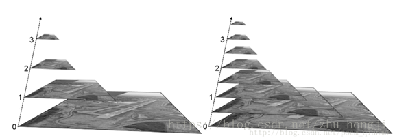
多分辨率采样图像,金字塔层级越高,图像越小,分辨率越低。
常见的两类金字塔,高斯金字塔(向下降采样),拉普拉斯laplacian金字塔(向上采样)
拉普拉斯金字塔仅限边缘图像,只要用于图像压缩,大多数元素为0

img = cv.imread('messi5.jpg')
# 向下采样,图像尺寸减半
lower_reso = cv.pyrDown(img)
lower_reso2 = cv.pyrDown(lower_reso)
lower_reso3 = cv.pyrDown(lower_reso2)
# 向上采样,图片尺寸扩大
higher_reso2 = cv.pyrUp(lower_reso3)
higher_reso3 = cv.pyrUp(higher_reso2)
higher_reso4 = cv.pyrUp(higher_reso3)
# 注意pyrDown和pyrUp并非逆操作,且两种处理均为非线性,不可逆且有损
8.2 使用金字塔进行图像融合
# 图像拼接中,使用金字塔进行图像融合可以无缝融合图像
A = cv.imread('apple.jpg')
B = cv.imread('orange.jpg')
# 为A生成6层高斯金字塔放在数组gpA中
G = A.copy()
gpA = [G]
for i in xrange(6):
    G = cv.pyrDown(G)
    gpA.append(G)
# 为B生成6层高斯金字塔放在数组gpB中
G = B.copy()
gpB = [G]
for i in xrange(6):
    G = cv.pyrDown(G)
    gpB.append(G)
# 在高斯金字塔基础上,为A生成拉普拉斯金字塔
lpA = [gpA[5]]
for i in xrange(5,0,-1):
    GE = cv.pyrUp(gpA[i])
    L = cv.subtract(gpA[i-1],GE)
    lpA.append(L)
# 在高斯金字塔基础上,为B生成拉普拉斯金字塔
lpB = [gpB[5]]
for i in xrange(5,0,-1):
    GE = cv.pyrUp(gpB[i])
    # 与前一张金字塔图像相减
    L = cv.subtract(gpB[i-1],GE)
    lpB.append(L)
# 每个级别中添加左右各一半的图像
LS = []
for la,lb in zip(lpA,lpB):
    rows,cols,dpt = la.shape
    # np.hstack()矩阵进行行连接
    ls = np.hstack((la[:,0:cols/2], lb[:,cols/2:]))
    LS.append(ls)
# 重建图像
ls_ = LS[0]
for i in xrange(1,6):
    ls_ = cv.pyrUp(ls_)
    ls_ = cv.add(ls_, LS[i])
# 图像各半边直接连接
real = np.hstack((A[:,:cols/2],B[:,cols/2:]))
cv.imwrite('Pyramid_blending2.jpg',ls_)
cv.imwrite('Direct_blending.jpg',real)

9. 轮廓
9.1 轮廓入门(寻找/绘制)
# cv.findContours(原图像,轮廓检索模式,轮廓逼近方法),返回修改后的图像、轮廓、层次
# 其中轮廓检索模式:
# 	cv::RETR_EXTERNAL:表示只提取最外面的轮廓;
# 	cv::RETR_LIST:表示提取所有轮廓并将其放入列表;
# 	cv::RETR_CCOMP:表示提取所有轮廓并将组织成一个两层结构,其中顶层轮廓是外部轮廓,第二层轮廓是“洞”的轮廓;
# 	cv::RETR_TREE:表示提取所有轮廓并组织成轮廓嵌套的完整层级结构
# 其中轮廓逼近方法:
# 	cv::CHAIN_APPROX_NONE:存储形状边界的所有点,如一条直线轮廓的所有点;
# 	cv::CHAIN_APPROX_SIMPLE:它删除所有冗余点并压缩轮廓,从而节省内存,如一条直线轮廓仅存储为两个点即可;
im = cv.imread('test.jpg')
# 将图片转化成灰度图
imgray = cv.cvtColor(im, cv.COLOR_BGR2GRAY)
# 全局简单阈值将图片从灰度图转为二值图像,ret=127,thresh为处理后的图像
ret, thresh = cv.threshold(imgray, 127, 255, 0)
# im2未返回
im2, contours, hierarchy = cv.findContours(thresh, cv.RETR_TREE, cv.CHAIN_APPROX_SIMPLE)
# cv.drawContours(原图像,轮廓python列表,轮廓索引,颜色厚度等)
# 注,若要绘制所有轮廓,则轮廓索引传-1
cv.drawContours(im, contours, -1, (0,255,0), 3) #绘制所有轮廓
cv.drawContours(im, contours, 3, (0,255,0), 3) #绘制第3个轮廓
cnt = contours[4]
cv.drawContours(im, [cnt], 0, (0,255,0), 3)
9.2 轮廓特征
# cv.moments(轮廓)计算图像的中心矩,用于提取轮廓相关信息
img = cv.imread('star.jpg',0)
ret,thresh = cv.threshold(img,127,255,0)
contours,hierarchy = cv.findContours(thresh, 1, 2)
cnt = contours[0]

M = cv.moments(cnt)
print( M )
# 由矩得到质心
cx = int(M['m10']/M['m00'])
cy = int(M['m01']/M['m00'])
# 轮廓区域面积--cv.contourArea
area = cv.contourArea(cnt) = M['m00']
# 轮廓区域周长
# cv.arcLength(轮廓,指定形状为闭合轮廓[true]或曲线)
perimeter = cv.arcLength(cnt,True)
# 轮廓近似
# cv.approxPolyDP(轮廓,轮廓到近似轮廓的最大距离,指定曲线是否闭合)
epsilon = 0.1*cv.arcLength(cnt,True)
approx = cv.approxPolyDP(cnt,epsilon,True)
# 求凸包的算法[Sklansky, J., Finding the Convex Hull of a Simple Polygon. PRL 1 $number, pp 79-83 (1982)]
# 求凸包cv.convexHull(凸包点集,输出的凸包点,bool凸包顺时针/逆时针)
hull = cv.convexHull(points[, hull[, clockwise[, returnPoints]]   hull = cv.convexHull(cnt)
凸包(Convex Hull)是一个计算几何(图形学)中的概念,在一个实数向量空间V中,对于给定集合X,所有包含X的凸集的交集S被称为X的凸包。 X的凸包可以用X内所有点(x1, x2….xn)的线性组合来构造。在二维欧几里得空间中,凸包可以想象为一条刚好包着所有点的橡皮圈,用不严谨的话来讲,给定二维平面上的点集,凸包就是将最外层的点连接起来构成的凸多边形,它能包含点集中所有的点。
returnPoints:默认为Ture。它会返回凸包上点的坐标。如果设置为False,就会返回与凸包点对应的轮廓上的点。


注意,轮廓与凸包的区别
# 检查曲线是否为凸形,返回true/false
k = cv.isContourConvex(cnt)

# 边界矩形
# 直边角矩形boundingRect,不考虑旋转,面积非最小,返回矩形左上角坐标(x,y)以及矩形的宽高(w,h)
x,y,w,h = cv.boundingRect(cnt)
cv.rectangle(img,(x,y),(x+w,y+h),(0,255,0),2)
# 获取最小外接矩阵,中心点坐标,宽高,旋转角度
rect = cv2.minAreaRect(points)
# 获取矩形四个顶点,浮点型
box = cv2.boxPoints(rect)
# 取整
box = np.int0(box)
# 画出轮廓
cv.drawContours(img,[box],0,(0,0,255),2)

# 外接圆
(x,y),radius = cv.minEnclosingCircle(cnt)
center = (int(x),int(y))
radius = int(radius)
# 画圆 cv.circle(原图像,中心点坐标,半径,颜色,粗细)
cv.circle(img,center,radius,(0,255,0),2)

# 拟合椭圆
# cv.fitEllipse()返回RotatedRect类型的值,通过一系列数学公式可以从RotatedRect获取到椭圆参数
ellipse = cv.fitEllipse(cnt)
# 画椭圆 cv.ellipse(原图像,椭圆参数,颜色,粗细)
cv.ellipse(img,ellipse,(0,255,0),2)

# 直线拟合
rows,cols = img.shape[:2]
# cv.fitLine(二维点数组,输出直线,距离类型,距离参数[0],径向精度参数[1e-2],角度精度参数[1e-2]),
[vx,vy,x,y] = cv.fitLine(cnt, cv.DIST_L2,0,0.01,0.01)
lefty = int((-x*vy/vx) + y)
righty = int(((cols-x)*vy/vx)+y)
# cv.line(原图像,直线起点,直线终点,颜色,粗细)
cv.line(img,(cols-1,righty),(0,lefty),(0,255,0),2)


9.3 轮廓属性
# 获取对象边界矩形的左上点坐标(x,y)和矩阵的宽高(w,h), 长宽比 aspect_ratio
x,y,w,h = cv.boundingRect(cnt)
aspect_ratio = float(w)/h

# 范围 = 轮廓面积/边界矩形区域面积
area = cv.contourArea(cnt)
x,y,w,h = cv.boundingRect(cnt)
rect_area = w*h
extent = float(area)/rect_area

# 坚固性 = 轮廓面积/凸包面积
area = cv.contourArea(cnt)
hull = cv.convexHull(cnt)
hull_area = cv.contourArea(hull)
solidity = float(area)/hull_area

# 等效直径 = 与轮廓面积等值的圆的直径
area = cv.contourArea(cnt)
equi_diameter = np.sqrt(4*area/np.pi)

# 方向,给出长轴长度MA和短轴长度ma
(x,y),(MA,ma),angle = cv.fitEllipse(cnt)

# 遮罩
mask = np.zeros(imgray.shape,np.uint8) #生成全0像素值的图像形状的遮罩
cv.drawContours(mask,[cnt],0,255,-1) #在遮罩上画出全部轮廓(白色)
pixelpoints = np.transpose(np.nonzero(mask)) #返回结果是构成图像的所有像素点
#pixelpoints = cv.findNonZero(mask)

# 使用遮罩图像可以得到最大值最小值及其位置
min_val, max_val, min_loc, max_loc = cv.minMaxLoc(imgray,mask = mask)

# 平均颜色和平均灰度
mean_val = cv.mean(im,mask = mask)

# 极点,对象最上/下/左/右边的点
leftmost = tuple(cnt[cnt[:,:,0].argmin()][0])
rightmost = tuple(cnt[cnt[:,:,0].argmax()][0])
topmost = tuple(cnt[cnt[:,:,1].argmin()][0])
bottommost = tuple(cnt[cnt[:,:,1].argmax()][0])
9.4 轮廓其他功能
9.4.1 凸缺陷
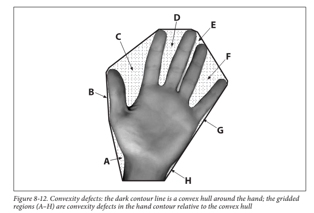
黑色的轮廓线为convexity hull, 而convexity hull与手掌之间的部分为convexity defects. 每个convexity defect区域有四个特征量:起始点(startPoint),结束点(endPoint),距离convexity hull最远点(farPoint),最远点到convexity hull的距离(depth)。
# cv.convexityDefects(轮廓[通过调用findContours得到],凸包[通过调用convexHull得到]),返回值包括(起始点、结束点、距离凸包最远点,最远点到凸包的距离)
img = cv.imread('star.jpg')
img_gray = cv.cvtColor(img,cv.COLOR_BGR2GRAY) #转为灰度图
ret,thresh = cv.threshold(img_gray, 127, 255,0) #变成二值图
contours,hierarchy = cv.findContours(thresh,2,1) #提取轮廓
cnt = contours[0]
# 注意,在寻找凸包时,必须传递returnPoints=False,取的是轮廓上的点
hull = cv.convexHull(cnt,returnPoints = False)
defects = cv.convexityDefects(cnt,hull)
for i in range(defects.shape[0]): #convexity defects(即夹缝区域)可能不止一个,所以轮流取
s,e,f,d = defects[i,0] #分别解析出每个convexity defects区域的四个值
start = tuple(cnt[s][0])
end = tuple(cnt[e][0])
far = tuple(cnt[f][0])
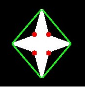
cv.line(img,start,end,[0,255,0],2) #绿色凸包,从起始点到终点(下图为例,应该有四个start-end)
cv.circle(img,far,5,[0,0,255],-1) #红色圆圈标识凸缺陷点,far为距离convexity hull最远点
cv.imshow('img',img)
cv.waitKey(0)
cv.destroyAllWindows()
9.4.2 点与轮廓的关系
# 查找图像中点与轮廓之间的最短距离,返回在轮廓外,距离为负,否则为正,在轮廓上则返回0.
dist = cv.pointPolygonTest(cnt,(50,50),True)
# cv.pointPolygonTest(轮廓、要检查的点,参数[True:返回带符号的距离,False:返回带符号的正负1和0])
9.4.3 比较两轮廓的形状
# cv.matchShapes(轮廓1,轮廓2,使用的比较方法,方法参数),返回值0-1,值越小说明匹配度越高。使用Hu矩(三种方法都使用了)特性:具有旋转,缩放和平移不变性
# CV_CONTOURS_MATCH_I1(标准矩)、CV_CONTOURS_MATCH_I2(p+q阶中心矩)、CV_CONTOURS_MATCH_I3(归一化中心矩)
img1 = cv.imread('star.jpg',0)
img2 = cv.imread('star2.jpg',0)
ret, thresh = cv.threshold(img1, 127, 255,0) #二值化
ret, thresh2 = cv.threshold(img2, 127, 255,0) #二值化
im2,contours,hierarchy = cv.findContours(thresh,2,1) #取轮廓
cnt1 = contours[0]
im2,contours,hierarchy = cv.findContours(thresh2,2,1) #取轮廓
cnt2 = contours[0]
ret = cv.matchShapes(cnt1,cnt2,1,0.0)
print( ret )
9.5 轮廓层次(即Contours中的父子关系)

0,1,2为第一层级、2a(2为外轮廓、2a为内轮廓)为第二层级、3是第三层级、3a为第四层、4和5(内层)为第五层。OpenCV表示层次结构,每层轮廓包含四个信息[Next、Previous、First_Child、Parent],注意某轮廓若为本层的第一个轮廓,则其Previous为-1;某轮廓若为本层的最后一个轮廓则其Next为-1;First_Child和Parent也是一样,若不存在则为-1。以2a为例子[Next=-1, Previous=-1, First_Child=3, Parent=2]
轮廓检索模式:
RETR_LIST:仅检索所有轮廓、不创建任何父子关系
RETR_EXTERNAL:仅返回最外部的轮廓,保留所有子轮廓不返回
RETA_CCOMP:仅排列为2级层次结构,外轮廓为一层,其余全部算作第二层轮廓,不再细分
RETR_TREE:检索所有轮廓及其层次列表

10. 直方图
10.1 直方图查找、绘制、分析
# 查找直方图
## OpenCV
# cv.calcHist(原图像、通道数[0/1/2分别计算蓝色/绿色/红色通道的直方图]、mask[若寻找图像特定区域的直方图,则需要创建遮罩图像作为mask,如全图则为None]、hitSize[bin的个数,总像素值为256,即直方图横坐标可以为0-256,也可将像素值等分成16份,0-15/16-31/...240-255之间的像素数,即直方图可以不用那么细化,则此时值为[16]]、范围[测量的强度值的范围,通常为0-256])
img = cv.imread('home.jpg',0)
hist = cv.calcHist([img],[0],None,[256],[0,256]) #注意参数都要用[]括起来
## Numpy
# 除了OpenCV外,Numpy也提供了直方图的计算查找np.histogram(待统计数据的数组、指定区间个数bin、范围[0-256]、weights数组每个元素的权重、density[true返回区间概率密度,false返回区间元素个数])
hist,bins = np.histogram(img.ravel(),256,[0,256])

# 绘制直方图
## 使用matplotlib——直接计算并绘制,无需调用calHist/histogram
img = cv.imread('home.jpg',0)
# matplotlib.pyplot.hist(数组、bins、range范围、normed归一化[true/false]、weights...)
plt.hist(img.ravel(),256,[0,256]);
plt.show()
## OpenCV
把直方图的值[y]和bin值[x]调整成x和y坐标,可以使用cv.line()、cv.polyline()

# Application of Mask
img = cv.imread('home.jpg',0)
# 创建一个格式为np.uint8的面具
mask = np.zeros(img.shape[:2], np.uint8)
mask[100:300, 100:400] = 255
masked_img = cv.bitwise_and(img,img,mask = mask)
hist_full = cv.calcHist([img],[0],None,[256],[0,256]) #计算不带mask的直方图
hist_mask = cv.calcHist([img],[0],mask,[256],[0,256]) #计算带mask的直方图
plt.subplot(221), plt.imshow(img, 'gray')
plt.subplot(222), plt.imshow(mask,'gray')
plt.subplot(223), plt.imshow(masked_img, 'gray')
plt.subplot(224), plt.plot(hist_full), plt.plot(hist_mask)
plt.xlim([0,256])
plt.show()


10.2 直方图均衡 (改善图像对比度)
若一个图像的像素值仅限于特定的值范围(例如,较亮的图像会将所有像素限制在较高的值。)但是,好的图像应该具有来自图像所有区域的像素。因此,您需要将此直方图拉伸到两端 (直方图均衡化,像素值分布更均匀广泛)。通常,这可以提高图像的对比度。
完美均衡的直方图,其累积直方图应为一条斜线

img = cv.imread('wiki.jpg',0)
hist,bins = np.histogram(img.flatten(),256,[0,256])# 返回值hist:数组直方图的值,bin:返回bin边缘(length(hist)+1)
cdf = hist.cumsum() # 计算累积直方图
cdf_normalized = cdf * float(hist.max()) / cdf.max() #均衡化直方图
plt.plot(cdf_normalized, color = 'b') #画累计直方图处理后的曲线
plt.hist(img.flatten(),256,[0,256], color = 'r') #绘制直方图
plt.xlim([0,256]) # x轴的范围
plt.legend(('cdf','histogram'), loc = 'upper left')
plt.show()

cdf_m = np.ma.masked_equal(cdf,0)
cdf_m = (cdf_m - cdf_m.min())*255/(cdf_m.max()-cdf_m.min())
cdf = np.ma.filled(cdf_m,0).astype('uint8')

img2 = cdf[img]

# OpenCV中直方图均衡 cv.equalizeHist(原图像,必须为灰度图),输出为直方图均衡图像
img = cv.imread('wiki.jpg',0)
equ = cv.equalizeHist(img)
res = np.hstack((img,equ)) #并排
cv.imwrite('res.png',res)

# 对于某些图像,如果直接对全图进行直方图均衡,可能由于亮度原因导致均衡后丢失某些信息,因此使用自适应直方图均衡【具体原理略】。
img = cv.imread('tsukuba_l.png',0)
# 创建一个CLAHE对象 (参数可选),cv.createCLAHE(颜色对比度阈值,在多少网格下进行直方图均衡化操作)实例化自适应直方图函数
clahe = cv.createCLAHE(clipLimit=2.0, tileGridSize=(8,8))
cl1 = clahe.apply(img) #进行自适应直方图均衡化操作
cv.imwrite('clahe_2.jpg',cl1)

[^直方图均衡图像]:


10.3 2D直方图
# OpenCV中,注意对于颜色直方图需要将图像从BGR转化为HSV,在一维直方图中,我们将BGR转化为灰度图
img = cv.imread('home.jpg')
hsv = cv.cvtColor(img,cv.COLOR_BGR2HSV)
# 参数为(hsv图像、通道[0,1]代表两个平面H和S、bins[H平面bins,S平面bins]、范围[H,S])
hist = cv.calcHist([hsv], [0, 1], None, [180, 256], [0, 180, 0, 256])

# Numpy提供的np.histogram2d(h数组、s数组、bins[H平面bins,S平面bins]、范围[H,S])
img = cv.imread('home.jpg')
hsv = cv.cvtColor(img,cv.COLOR_BGR2HSV)
hist, xbins, ybins = np.histogram2d(h.ravel(),s.ravel(),[180,256],[[0,180],[0,256]])

#绘制直方图
img = cv.imread('home.jpg')
hsv = cv.cvtColor(img,cv.COLOR_BGR2HSV)
hist = cv.calcHist( [hsv], [0, 1], None, [180, 256], [0, 180, 0, 256] )
plt.imshow(hist,interpolation = 'nearest') #绘图时使用插值标记可以得到较好的结果
plt.show() #x轴得到S值,y轴得到H值

10.4 直方图反投影 (用于图像分割或在图像中找到感兴趣的对象)
# Numpy中的算法
#roi是我们感兴趣的对象,要找到的对象
roi = cv.imread('rose_red.png')
hsv = cv.cvtColor(roi,cv.COLOR_BGR2HSV)
#target是我们要搜索的对象
target = cv.imread('rose.png')
hsvt = cv.cvtColor(target,cv.COLOR_BGR2HSV)
# 分别找到两者的2D直方图
M = cv.calcHist([hsv],[0, 1], None, [180, 256], [0, 180, 0, 256] )
I = cv.calcHist([hsvt],[0, 1], None, [180, 256], [0, 180, 0, 256] )
# 第二是找到比率R=M/I,然后反投影R,即使用R作为调色板,并创建一个新图像
R = M / I
h,s,v = cv.split(hsvt)
B = R[h.ravel(),s.ravel()]  # h是色相,s是像素(x,y)处的饱和度
B = np.minimum(B,1)
B = B.reshape(hsvt.shape[:2])
# 现在应用和圆盘的卷积,B=D*B,其中D是卷积核
disc = cv.getStructuringElement(cv.MORPH_ELLIPSE,(5,5))
cv.filter2D(B,-1,disc,B)
B = np.uint8(B)
cv.normalize(B,B,0,255,cv.NORM_MINMAX)
ret,thresh = cv.threshold(B,50,255,0) #现在最大强度的位置即是物体的位置。如果我们期待图像中的某个区域,则为合适的值设置阈值会给出更好的结果

# OpenCV中的算法
roi = cv.imread('rose_red.png')
hsv = cv.cvtColor(roi,cv.COLOR_BGR2HSV)
target = cv.imread('rose.png')
hsvt = cv.cvtColor(target,cv.COLOR_BGR2HSV)
# 计算目标直方图
roihist = cv.calcHist([hsv],[0, 1], None, [180, 256], [0, 180, 0, 256] )
# 规格化直方图并应用反射投影
cv.normalize(roihist,roihist,0,255,cv.NORM_MINMAX)
# cv.calcBackProject(原图像、通道列表[H,S]、输入直方图、直方图对应范围)
dst = cv.calcBackProject([hsvt],[0,1],roihist,[0,180,0,256],1)
# cv.getStructuringElement(内核形状、内核尺寸、锚点位置),返回指定形状和尺寸的结构元素
disc = cv.getStructuringElement(cv.MORPH_ELLIPSE,(5,5)) #椭圆
# 核的中心对准源图像的像素,源图像和核的相对应元素分别相乘并全部相加,得到的值为目标图像核心的值,用上面生成的椭圆核(原图像、目标图像所需深度、卷积核、核锚点)
cv.filter2D(dst,-1,disc,dst)
# 设置阈值与二进制AND
ret,thresh = cv.threshold(dst,50,255,0)
thresh = cv.merge((thresh,thresh,thresh))
res = cv.bitwise_and(target,thresh)
res = np.vstack((target,thresh,res))
cv.imwrite('res.jpg',res)
11 傅里叶变换
图像处理一般分为空间域处理和频率域处理
空间域处理是直接对图像内的像素进行处理。主要划分为灰度变换核空间滤波两种形式,
灰度变换对图像内的单个像素进行处理,滤波处理涉及对图像质量的改变
频率域处理是先将图像变换到频率域,然后在频率域对图像进行处理,最后通过反变换将图像变为空间域。
傅里叶变换可以将图像变换为频率域, 傅立叶反变换将频率域变换为空间域
# Numpy中的傅里叶变换
# 在模块numpy中fft2()就是傅里叶变换的简单函数,首先我们以灰度模式读入图像,在imread()函数中参数中,0代表灰度模式,读入以后用fft2函数,将读入的数据进行傅里叶变换,输出结果为复数形式
img = cv.imread('messi5.jpg',0)
f = np.fft.fft2(img)
fshift = np.fft.fftshift(f) #图像中心化处理,即把低频白色部分往中间移动
magnitude_spectrum = 20*np.log(np.abs(fshift)) # 结果是复数,求绝对值才是振幅

# 设置高通滤波器
rows, cols = img.shape
crow,ccol = rows//2 , cols//2
fshift[crow-30:crow+31, ccol-30:ccol+31] = 0

# 傅里叶逆变换
f_ishift = np.fft.ifftshift(fshift) #fftshit()函数的逆函数,它将频谱图像的中心低频部分移动至左上角
img_back = np.fft.ifft2(f_ishift) #实现图像逆傅里叶变换,返回一个复数数组
img_back = np.real(img_back)

plt.subplot(131),plt.imshow(img, cmap = 'gray')
plt.title('Input Image'), plt.xticks([]), plt.yticks([])
plt.subplot(132),plt.imshow(img_back, cmap = 'gray')
plt.title('Image after HPF'), plt.xticks([]), plt.yticks([])
plt.subplot(133),plt.imshow(img_back)
plt.title('Result in JET'), plt.xticks([]), plt.yticks([])
plt.show()
# OpenCV中的傅里叶变换
img = cv.imread('messi5.jpg',0)
# 傅里叶变换  cv2.DFT_COMPLEX_OUTPUT 执行一维或二维复数阵列的逆变换,结果通常是相同大小的复数数组
dft = cv.dft(np.float32(img),flags = cv.DFT_COMPLEX_OUTPUT)
dft_shift = np.fft.fftshift(dft) #图像中心化处理
magnitude_spectrum = 20*np.log(cv.magnitude(dft_shift[:,:,0],dft_shift[:,:,1])) # 频谱图像双通道复数转换为0~255区间

# 设置低通滤波器
rows, cols = img.shape
crow,ccol = rows/2 , cols/2
mask = np.zeros((rows,cols,2),np.uint8)
mask[crow-30:crow+30, ccol-30:ccol+30] = 1
fshift = dft_shift*mask #mask与频谱图像乘积

# 傅里叶逆变换
f_ishift = np.fft.ifftshift(fshift)
img_back = cv.idft(f_ishift)
img_back = cv.magnitude(img_back[:,:,0],img_back[:,:,1])
plt.subplot(121),plt.imshow(img, cmap = 'gray')
plt.title('Input Image'), plt.xticks([]), plt.yticks([])
plt.subplot(122),plt.imshow(img_back, cmap = 'gray')
plt.title('Magnitude Spectrum'), plt.xticks([]), plt.yticks([])
plt.show()
12 模板匹配 (在较大图像中搜索和查找模板图像位置的方法)
img = cv.imread('messi5.jpg',0)
img2 = img.copy()
template = cv.imread('template.jpg',0) #模板
w, h = template.shape[::-1]
# 6种比较方法
methods = ['cv.TM_CCOEFF', 'cv.TM_CCOEFF_NORMED', 'cv.TM_CCORR',
            'cv.TM_CCORR_NORMED', 'cv.TM_SQDIFF', 'cv.TM_SQDIFF_NORMED']
for meth in methods:
    img = img2.copy()
    method = eval(meth)
    # 模板匹配cv.matchTemplate(原图像、模板图像、比较方法)
    res = cv.matchTemplate(img,template,method)
    min_val, max_val, min_loc, max_loc = cv.minMaxLoc(res)#cv.minMaxLoc()函数查找最大/最小值在哪
    # 如果方法是TM_SQDIFF或TM_SQDIFF_NORMED,则取最小值,得到top_left矩形的左上角,并以(w,h) 作为矩形的宽度和高度。该矩形就是模板的区域。
    if method in [cv.TM_SQDIFF, cv.TM_SQDIFF_NORMED]:
        top_left = min_loc
    else:
        top_left = max_loc
    bottom_right = (top_left[0] + w, top_left[1] + h)
    cv.rectangle(img,top_left, bottom_right, 255, 2) #画出矩形
    plt.subplot(121),plt.imshow(res,cmap = 'gray')
    plt.title('Matching Result'), plt.xticks([]), plt.yticks([])
    plt.subplot(122),plt.imshow(img,cmap = 'gray')
    plt.title('Detected Point'), plt.xticks([]), plt.yticks([])
    plt.suptitle(meth)
    plt.show()

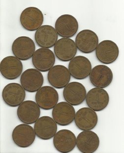
# 多对象模板匹配
img_rgb = cv.imread('mario.png')
img_gray = cv.cvtColor(img_rgb, cv.COLOR_BGR2GRAY)
template = cv.imread('mario_coin.png',0)
w, h = template.shape[::-1]
res = cv.matchTemplate(img_gray,template,cv.TM_CCOEFF_NORMED)
threshold = 0.8 #加入threshold阈值,可以调整包含对象的概率
loc = np.where( res >= threshold) #函数np.where()可以找出在函数cv2.matchTemplate()的返回值(图像)中,哪些位置上的值是大于阈值threshold的
for pt in zip(*loc[::-1]):
    cv.rectangle(img_rgb, pt, (pt[0] + w, pt[1] + h), (0,0,255), 2)
cv.imwrite('res.png',img_rgb)

13 霍夫变换 (Hough变换是图像处理中从图像中识别几何形状的基本方法之一)
13.1 霍夫线变换
# cv.HoughLines(输入图像[灰度图]、像素扫描步长、角度步长、阈值[获得足够交点的极坐标点才被看成是直线]),输出为极坐标(r,theta)表示直线。
img = cv.imread(cv.samples.findFile('sudoku.png'))
gray = cv.cvtColor(img,cv.COLOR_BGR2GRAY)
edges = cv.Canny(gray,50,150,apertureSize = 3)
lines = cv.HoughLines(edges,1,np.pi/180,200)
for line in lines: #返回多条直线
    rho,theta = line[0]
    a = np.cos(theta)
    b = np.sin(theta)
    x0 = a*rho
    y0 = b*rho
    x1 = int(x0 + 1000*(-b))
    y1 = int(y0 + 1000*(a))
    x2 = int(x0 - 1000*(-b))
    y2 = int(y0 - 1000*(a))
    cv.line(img,(x1,y1),(x2,y2),(0,0,255),2)
cv.imwrite('houghlines3.jpg',img)
# cv.HoughLinesP(输入图像[灰度图]、像素扫描步长、角度步长、阈值、minLineLength最小直线长度、maxLineGap最大间隔),输出为极坐标(r,theta)表示直线
img = cv.imread(cv.samples.findFile('sudoku.png'))
gray = cv.cvtColor(img,cv.COLOR_BGR2GRAY)
edges = cv.Canny(gray,50,150,apertureSize = 3)
lines = cv.HoughLinesP(edges,1,np.pi/180,100,minLineLength=100,maxLineGap=10)
for line in lines:
    x1,y1,x2,y2 = line[0]
    cv.line(img,(x1,y1),(x2,y2),(0,255,0),2)
cv.imwrite('houghlines5.jpg',img)


13.2 霍夫圆变换
# 霍夫圆检测对噪声比较敏感,所以首先要对图像做滤波处理,Opencv中实现的霍夫变换圆检测是基于图像梯度的实现,分为两步:1. 检测边缘,发现可能的圆心; 2. 基于第一步的基础上从候选圆心开始计算最佳半径大小
# cv.HoughCircles(输入图像[8位单通道灰度图]、方法、dp、mindist、param1[Canny边缘检测最低阈值]、param2[候选圆心]、最小半径、最大半径)
img = cv.imread('opencv-logo-white.png',0)
img = cv.medianBlur(img,5)
cimg = cv.cvtColor(img,cv.COLOR_GRAY2BGR)
circles = cv.HoughCircles(img,cv.HOUGH_GRADIENT,1,20,
                            param1=50,param2=30,minRadius=0,maxRadius=0)
circles = np.uint16(np.around(circles))
for i in circles[0,:]:
    cv.circle(cimg,(i[0],i[1]),i[2],(0,255,0),2) #画外圈
    cv.circle(cimg,(i[0],i[1]),2,(0,0,255),3) #画圆心
cv.imshow('detected circles',cimg)
cv.waitKey(0)
cv.destroyAllWindows()

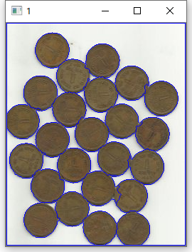
14 分水岭算法的图像分割
img = cv.imread('coins.png')
gray = cv.cvtColor(img,cv.COLOR_BGR2GRAY) #颜色转化
ret, thresh = cv.threshold(gray,0,255,cv.THRESH_BINARY_INV+cv.THRESH_OTSU) #Otsu二值化
# 去除噪声
kernel = np.ones((3,3),np.uint8) #生成卷积核
opening = cv.morphologyEx(thresh,cv.MORPH_OPEN,kernel, iterations = 2) #2次开运算,[形态变化,先腐蚀,再膨胀,可清除一些小东西(亮的),放大局部低亮度的区域]
# 确定背景区域
sure_bg = cv.dilate(opening,kernel,iterations=3) #对输入图像用特定结构元素进行膨胀操作,各点像素值将被替换为对应邻域上的最大值
# 确定前景区域
	# 距离变换的基本含义是计算一个图像中非零像素点到最近的零像素点的距离,
    # 也就是到零像素点的最短距离
    # 个最常见的距离变换算法就是通过连续的腐蚀操作来实现,腐蚀操作的停止条件是所有前景像素都被完全腐蚀。
    # 这样根据腐蚀的先后顺序,我们就得到各个前景像素点到前景中心像素点的距离。
    # 根据各个像素点的距离值,设置为不同的灰度值。这样就完成了二值图像的距离变换
    # cv.distanceTransform(二值图、距离类型、maskSize)[计算二值图像内任意点到最近背景点的距离; 输出的是保存每一个非零点与最近零点的距离信息;图像上越亮的点,代表了离零点的距离越远。可以方便地将前景对象提取出来。]
    # 第二个参数 0,1,2 分别表示 CV_DIST_L1, CV_DIST_L2 , CV_DIST_C
dist_transform = cv.distanceTransform(opening,cv.DIST_L2,5)
ret, sure_fg = cv.threshold(dist_transform,0.7*dist_transform.max(),255,0)
# 找出未知区域
sure_fg = np.uint8(sure_fg)
unknown = cv.subtract(sure_bg,sure_fg)
# 找出连通区域(类别标记)
ret, markers = cv.connectedComponents(sure_fg)
# 将所有标记加1,保证不是背景的标记不是0
markers = markers+1
# 让所有未知区域记为 0
markers[unknown==255] = 0
# 分水岭算法, 边界区域置为 -1
markers = cv.watershed(img,markers)
img[markers == -1] = [255,0,0]
15 GrabCut算法进行交互式前景提取 (把物体和其背景分离)
# 原理:首先[矩形框选法]先把这个图片的前景部分用矩形圈起来,默认框里面的有背景有前景物体,框外全是背景。下一步建立一个和图片等大的mask,初始全0,计算后可以标识背景和前景[背景<前景],
img = cv.imread('messi5.jpg')
mask = np.zeros(img.shape[:2],np.uint8) #建立一个和img图像一样大的蒙版
bgdModel = np.zeros((1,65),np.float64)
fgdModel = np.zeros((1,65),np.float64)
rect = (50,50,450,290)
cv.grabCut(img,mask,rect,bgdModel,fgdModel,5,cv.GC_INIT_WITH_RECT)
mask2 = np.where((mask==2)|(mask==0),0,1).astype('uint8')
img = img*mask2[:,:,np.newaxis]
plt.imshow(img),plt.colorbar(),plt.show()

# newmask is the mask image I manually labelled
newmask = cv.imread('newmask.png',0)
# wherever it is marked white (sure foreground), change mask=1
# wherever it is marked black (sure background), change mask=0
mask[newmask == 0] = 0
mask[newmask == 255] = 1
mask, bgdModel, fgdModel = cv.grabCut(img,mask,None,bgdModel,fgdModel,5,cv.GC_INIT_WITH_MASK)
mask = np.where((mask==2)|(mask==0),0,1).astype('uint8')
img = img*mask[:,:,np.newaxis]
plt.imshow(img),plt.colorbar(),plt.show()