RANSAC是提升模型估计鲁棒性一个经典的算法,被用在很多计算机视觉应用。但是目前为止,把RANSAC当作深度学习pipeline一个组成部分的方法还没有,原因是RANSAC选择hypothesis的步骤, 不可求导。这篇论文中,设计了两种方法,让RANSAC选择hypothesis的步骤可导。其中最有前景的方法受到了强化学习的启发,就是把 deterministic hypothesis selection 替换为 probabilistic selection,这样就能求损失函数对模型中的所有可学习参数的导数,进而把RANSAC和深度学习结合起来。这种方法叫作 Differentiable RANSAC(DSAC)。 本文做了一个示例,把DSAC应用于 Camera Localization,实验证明把RANSAC和深度学习结合起来直接估计相机姿态,能够达到更高的准确性。文章同时认为DSAC可嵌入其他深度学习任务。
文章标题:DSAC - Differentiable RANSAC for Camera Localization
文章作者:Eric Brachmann, Alexander Krull, Sebastian Nowozin(来自TU Dresden、微软)
收录情况:CVPR 2017
回顾RANSAC
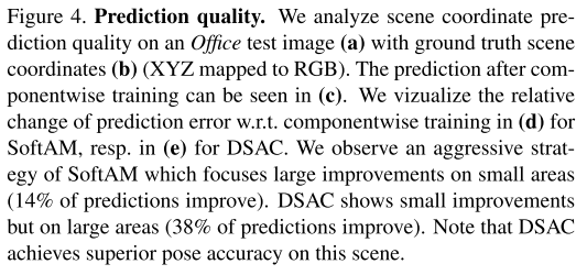
用一个简单例子说明:有一个点集P,现在想用一条直线拟合这个点集,使得这条直线最能反映点的分布情况。RANSAC解决此问题方法如下:
- 设定迭代次数 k,误差阈值$\tau$
- 第i次迭代:
- 从点集随机取2个点,这2个点组成了minimal set(因为两点就能确定一条直线),用minimal set计算模型参数(斜率a和截距b)—— current hypothesis
- 计算点集P中所有点与 current hypothesis 的误差,确定 inlier set
- 输出最大 inlier set 对应的模型
简介
random sample consensus(RANSAC)1981年提出以来,在robust estimation方面产生了很大影响力,它能处理带有许多离群值的数据,并且容易实现。基于RANSAC的研究工作不断出现,应用到了计算机视觉的很多领域:multi-view geometry/ object retrieval/ pose estimation/ SLAM。这些应用有一个共同点:从局部预测得到全局模型,而RANSAC能纠正局部预测的一些错误,从而产生鲁棒的结果。
相关工作
- RANSAC 变体(都是很早之前的工作了)
- M. A. Fischler and R. C. Bolles. Random sample consen- sus: A paradigm for model fitting with applications to image analysis and automated cartography. Commun. ACM, 1981.
- O. Chum and J. Matas. Matching with prosac ” progressive sample consensus. In CVPR, 2005.
- O. Chum, J. Matas, and J. Kittler. Locally Optimized RANSAC. 2003.
- D. Nist´er. Preemptive ransac for live structure and motion estimation. In ICCV, 2003.
- P. H. S. Torr and A. Zisserman. MLESAC: A new robust esti- mator with application to estimating image geometry. CVIU, 2000.
- R. Raguram, J.-M. Frahm, and M. Pollefeys. A comparative analysis of ransac techniques leading to adaptive real-time random sample consensus. In ECCV, 2008.
- Differentiable Algorithms in CNN
- J. Long, E. Shelhamer, and T. Darrell. Fully convolutional networks for semantic segmentation. In CVPR, 2015.
- D. Eigen and R. Fergus. Predicting depth, surface normals and semantic labels with a common multi-scale convolu- tional architecture.
- M. D. Zeiler and R. Fergus. Visualizing and understanding convolutional networks. In ECCV, 2014.
- A. Krizhevsky, I. Sutskever, and G. E. Hinton. Imagenet classification with deep convolutional neural networks. In NIPS, 2012.
- D. G. Lowe. Distinctive image features from scale-invariant keypoints. IJCV, 2004.
- J. Revaud, P. Weinzaepfel, Z. Harchaoui, and C. Schmid. Deepmatching: Hierarchical deformable dense matching. IJCV, 2016.
- S. Shalev-Shwartz and A. Shashua. On the sample complex- ity of end-to-end training vs. semantic abstraction training. CoRR, 2016.
- K. M. Yi, E. Trulls, V. Lepetit, and P. Fua. Lift: Learned invariant feature transform. In ECCV, 2016.
- R. Arandjelovi´c, P. Gronat, A. Torii, T. Pajdla, and J. Sivic. NetVLAD: CNN architecture for weakly supervised place recognition. In CVPR, 2016.
- R. Arandjelovic and A. Zisserman. All about vlad. In CVPR, 2013.
- J. Schulman, N. Heess, T. Weber, and P. Abbeel. Gradient estimation using stochastic computation graphs. In NIPS, 2015.
- Camera Localiztion
- J. Shotton, B. Glocker, C. Zach, S. Izadi, A. Criminisi, and A. Fitzgibbon. Scene coordinate regression forests for cam- era relocalization in rgb-d images. In CVPR, 2013.
- A. Guzman-Rivera, P. Kohli, B. Glocker, J. Shotton, T. Sharp, A. Fitzgibbon, and S. Izadi. Multi-output learn- ing for camera relocalization. In CVPR, 2014.
- J. Valentin, M. Nießner, J. Shotton, A. Fitzgibbon, S. Izadi, and P. H. S. Torr. Exploiting uncertainty in regression forests for accurate camera relocalization. In CVPR, 2015.
- E. Brachmann, F. Michel, A. Krull, M. Y. Yang, S. Gumhold, and C. Rother. Uncertainty-driven 6d pose estimation of ob- jects and scenes from a single rgb image. In CVPR, 2016.
- A. Krull, E. Brachmann, F. Michel, M. Y. Yang, S. Gumhold, and C. Rother. Learning analysis-by-synthesis for 6d pose estimation in rgb-d images. In ICCV, 2015.
- A. Kendall, M. Grimes, and R. Cipolla. Posenet: A convolu- tional network for real-time 6-dof camera relocalization. In ICCV, 2015.
主要方法
 本文把DSAC应用到”相机定位”问题。 相机位姿有6个自由度,即3个旋转自由度 + 3个平移自由度,这些自由度以真实世界坐标系(scene’s coordinate frame,3D坐标系)为参考。
- 问题定义:对于RGB图片I,目标是估计参数$\tilde{\textbf{h}}$,使得2D-3D空间如下转换关系成立
- \[Y(I) = \{\textbf{y}(I, i)|\forall i\}\]
- $\textbf{y}(I, i)$是像素$i$在世界坐标系的位置。
- 下文中,用$\textbf{y}_i$表示$\textbf{y}(I, i)$,用$Y(I)$表示图片I所有像素点的世界坐标系位置集合。再用$Y$表示$Y(I)$。
- 用RANSAC从$Y$估计$\tilde{\textbf{h}}$的步骤如下:
- 生成hypotheses集合。生成一个hypothesis时,从$Y(I)$中挑选一个 minimal set,\(Y_J, J = \{j_1, j_2, \cdots, j_n\}\),$n$是minimal set元素个数。从2D-3D的对应关系均匀采样,样本索引 \(j_m \in \{1,\cdots,\|Y\|\}\),以此得到$Y_J$。假设函数$\textbf{H}$,使得\(\textbf{h}_J = \textbf{H}(Y_J)\)成立。在相机定位问题中,$\textbf{H}$是 perspective-n-point(PNP) 算法。
- 对集合中的hypothesis打分。标量值函数 $s(\textbf{h}_J, Y)$评估$\textbf{h}_J$的consensus——可以用inlier set元素个数评价。
这里用3D世界坐标$\textbf{y}_i$的重投影误差判断inlier point
- \[e_i = || \textbf{p}_i - C\textbf{h}_J\textbf{y}_i ||\]
- $\textbf{p}_i$ 是像素i的2D位置,$C$是相机重投影矩阵
- 当$e_i < \tau$时,$\textbf{y}_i$视作一个 inlier
- IMPORTANT:这篇论文不去计数 inlier,而是根据$e_i$用 $s(\textbf{h}_J, Y) 计算 hypothesis 得分
- 选择最好的hypothesis。
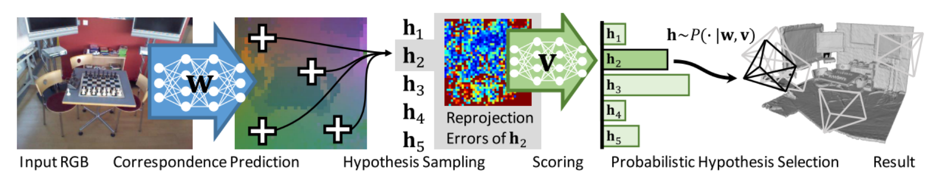
- \[\textbf{h}_{AM} = argmax_{\textbf{h}_{J}} ~s(\textbf{h}_J, Y)\]
- 进一步优化hypothesis。
- 优化函数 \(\textbf{R}(\textbf{h}_{AM}, \textbf{Y})\)
- $\textbf{R}$可能用上所有的2D-3D对应关系$Y$,一种常用的做法是从$Y$选一个内点集,用这个内点集重新计算函数 $\textbf{H}$
- 最后的输出 \(\tilde{\textbf{h}}_{AM} = \textbf{R}(\textbf{h}_{AM}, \textbf{Y})\)
- 用神经网络的方法学习RANSAC中hypothesis的参数
- 本文的目标是同时学习两个函数:$\textbf{y}(I,i;\textbf{w})$和$s(\textbf{h}_J,Y;\textbf{v})$,$\textbf{w}$(影响相机姿态)和$\textbf{v}$(影响hypothesis选择)是其中的参数
- 记$\textbf{Y}^{\textbf{w}}$,表明相机3D坐标预测依赖参数$\textbf{w}$;记$\textbf{Y}^{\textbf{w},\textbf{v}}_{AM}$,表明hypothesis选择依赖参数$\textbf{w}$、$\textbf{v}$
- 优化$\textbf{w}、\textbf{v}$,使得
- \[\tilde{\textbf{w}}, \tilde{\textbf{v}} = argmin_{\textbf{w},\textbf{v}} \sum_{I \in \mathcal{I}} \mathcal{l}(\textbf{R}(\textbf{h}_{AM}^{\textbf{w},\textbf{v}}, \textbf{Y}^{\textbf{w}}), \textbf{h}^{\star})\]
- $h^{*}$ 是$I$的 ground truth 模型参数
- 为了能端到端的神经网络学习,损失函数需要对 $\textbf{w},\textbf{v}$ 可导
- Soft argmax Selection(SoftAM)
- 选择最好的hypothesis时,\(\textbf{h}_{AM} = argmax_{\textbf{h}_{J}} ~s(\textbf{h}_J, Y)\)这种形式是不可导的,一种思路是把 argmax 替换成 soft argmax,即对hypotheses加权平均
- \[\textbf{h}^{\textbf{w}, \textbf{v}}_{SoftAM} = \sum_{J} P(J\|\textbf{w}, \textbf{v}) \textbf{h}_{J}^{\textbf{w}}\]
- \[P(J\|\textbf{w}, \textbf{v}) = \frac{\exp(s(\textbf{h}_{J}^{\textbf{w}}, Y^{\textbf{w}}; \textbf{v}))}{\sum_{J'} \exp(s(\textbf{h}_{J'}^{\textbf{w}}Y^{\textbf{w}};\textbf{v}))}\]
- hypothesis 变成这种形式时,迫使打分函数 $s(\textbf{h}_{J}^{\textbf{w}}, Y^{\textbf{w}}; \textbf{v})$ 预测的模型参数更鲁棒(???何以见得)$\Rightarrow$ 离群样本对应的模型参数权重很小,这样才不会影响\(\textbf{h}^{\textbf{w}, \textbf{v}}_{SoftAM}\)的准确性
- 使用 soft argmax,背离了 RANSAC 的原则:making one hard decision for a hypothesis(没懂在说什么?)
- 使用 soft argmax 做hypothesis选择,与鲁棒优化领域的独立应变具有相似性(???翻译过来有些生搬硬套),独立应变指 robust averaging
- 下面介绍另一种hypothesis selection方案:Probabilistic Selection
- 选择最好的hypothesis时,\(\textbf{h}_{AM} = argmax_{\textbf{h}_{J}} ~s(\textbf{h}_J, Y)\)这种形式是不可导的,一种思路是把 argmax 替换成 soft argmax,即对hypotheses加权平均
- Probabilistic Selection(DSAC)
- 选择 hypothesis 时根据如下方法
- \(\textbf{h}^{\textbf{w}, \textbf{v}}_{DSAC} = \textbf{h}_{J}^{\textbf{w}}\),with $J \sim P(J|\textbf{v}, \textbf{w})$
- $P(J|\textbf{v}, \textbf{w})$ 与 soft argmax selection 中的计算方法一致,是$s(\textbf{h}_{J}^{\textbf{w}}; \textbf{v})$ 的softmax分布
- 这种方法的灵感来自于 reinforcement learning —— 最小化定义在 stochastic process 的损失函数
- 学习 $\textbf{w}, \textbf{v}$ 时,最小化随机过程损失函数的期望
- \[\tilde{\textbf{w}}, \tilde{\textbf{v}} = argmin_{\textbf{w}, \textbf{v}} \sum_{I \in \mathcal{I}} \mathbb{E}_{J \sim P(J\|\textbf{w},\textbf{v})} [\mathcal{l}(\textbf{R}(\textbf{h}_{J}^{\textbf{w}}, Y^{\textbf{w}}))]\]
- 上式对于$\textbf{w}$的导数,可以表示为
- \[\frac{\partial}{\partial \textbf{w}} \mathbb{E}_{J \sim P(J\|\textbf{v}, \textbf{w})} [\mathcal{l}(\cdot)] = \mathbb{E}_{J \sim P(J\|\textbf{v}, \textbf{w})} \left[ \mathcal{l}(\cdot)\frac{\partial}{\partial \textbf{w}} \log{P(J\|\textbf{v}, \textbf{w})} + \frac{\partial}{\partial \textbf{w}} \mathcal{l}(\cdot) \right]\]
- 对于$\textbf{v}$的导数,可用类似的方法求
- 这种方法就是 DSAC:Differentiable SAmple Consensus
- 选择 hypothesis 时根据如下方法
- Differentiable Camera Localzation
-
整个方法的设计受到了这篇文章的启发 “E. Brachmann, F. Michel, A. Krull, M. Y. Yang, S. Gumhold, and C. Rother. Uncertainty-driven 6d pose estimation of ob- jects and scenes from a single rgb image. In CVPR, 2016.”
-
上面这篇文章是对 SCoRF 的扩展工作,from RGB-D to RGB images
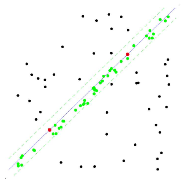
- 具体的pipeline:
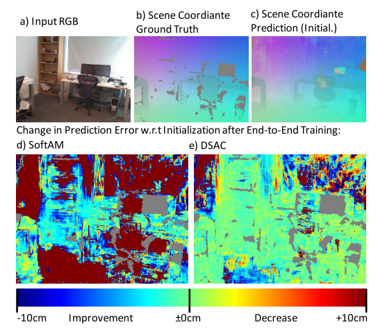
- 用一个CNN预测 像素点在真实空间的位置。每个 42x42 pixel image patch,预测一个 scene coordinate point;每幅图像预测 40x40 个这样的patch
- 用另一个CNN给hypotheses打分——基于重投影误差。对于每个预测的 scene coordinate $\textbf{y}_i$,计算对应$\textbf{h}_J$的重投影误差$e_i$
- Instead of the preemptive RANSAC schema, we score hypotheses only once and select the final pose, either by applying the soft argmax operator (SoftAM), or by probabilistic selection according to the softmaxed scores (DSAC).
- Only the final pose is refined. We choose inlier object coordinate predictions (at most 100), i.e. scene coordinates yi with reprojection error $e_i$ < $\tau$, and solve PNP [24] again using this set. This is iterated multiple times. Since the Coordinate CNN predicts only point estimates we do no further pose optimization using uncertainty.
实验
- 数据集:7-Scenes
- 7个室内环境的RGB-D图像,每帧图像带有相机位姿标注——6个自由度
- 每个场景的3D模型已知
- 每个场景由多个image sequences组成,数量从1k~7k不等,可能被用作train,也可能test
- 本文做实验的时候,忽略掉了RGB-D深度值这个channel,仅用RGB图片估计相机位姿
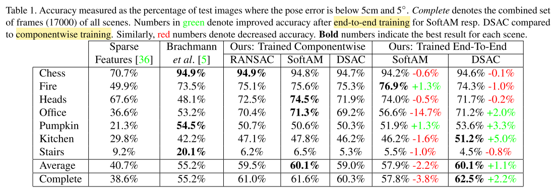
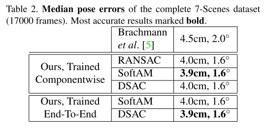
- 评价指标:相机姿态误差小于5°和5cm的图片的百分比
- 训练时,采用可导的损失函数:
- \[\mathcal{l}_{pose}(\textbf{h}, \boldsymbol{h^{*}}) = \max(\measuredangle (\boldsymbol{\theta},\boldsymbol{\theta^{*}}), \parallel \textbf{t} - \textbf{t}^{*} \parallel)\]