AlexNet

今天分享的这篇论文发表时间是2012年，算是比较早了，是把深度卷积神经网络成功应用在计算机视觉领域的开山之作，目前被引用量接近 70000，可见影响力非常之大，可以说做视觉的论文十有八九会引用它。网络上对它的讲解非常之多，再拿出来阅读，是因为它很经典，搞清楚深度卷积神经网络一些最基本的东西。

论文标题：ImageNet Classification with Deep Convolutional Neural Networks
论文作者：Alex Krizhevsky, Ilya Sutskever, Geoffrey E. Hinton（多伦多大学）
收录情况：NIPS 2012

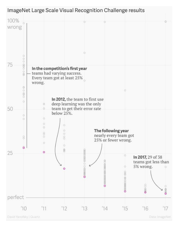
这篇论文提出的神经网络被称为 AlexNet，它的成名源于一个视觉识别竞赛 ImageNet Large Scale Vision Recognition Challenge (ILSVRC)——2010年开办，每年一次，2017年年结束。ImageNet是一个计算机视觉领域的公开数据集，规模非常之大——涵盖22000个类别的1500万张标注图片，目的是让研究人员的算法在上面做实验，

Image Classification
Object Detection
Semantic Segmentation

比较不同算法的优劣，促进视觉研究的进步。ILSVRC 使用的是 ImageNet 的一部分数据，包含~120万张图片，分成1000类，每类~1200张图片，划分成训练集（100万张标注图片）、验证集（5万张标注图片，用于自己评估算法效果）、测试集（15万张无标签图片，预测结果提交到主办方评估）参赛者需要开发算法把测试集图片分到正确的类别。这其实是个比较困难的任务。

简介

AlexNet 是一个8层的神经网络，5个卷积层 + 3个全连接层
几个创新点 —— 现在看来是 tricks：
- 激活函数使用 ReLU
- 分布式训练 —— 使用了两块GPU
- 使用 Normalization
- 使用 Overlapping Pooling
- Dropout 应用到了全连接层
现在看似很简单，实际上经历了长期探索

模型结构

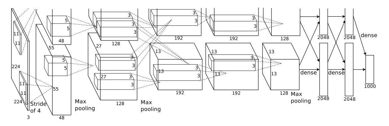
输入：224 x 224 的RGB图片
输出：1000维的向量，每维表示对应类别的概率
参数量计算
- 对于AlexNet：模型参数只存在于卷积层、全连接层
- 一些预备知识
  - $O_w = \lfloor \frac{I_w - k_w + 2P_w}{s_w} \rfloor$ + 1；$O_h = \lfloor \frac{I_h - k_h + 2P_h}{s_h} \rfloor$ + 1
  - $I_w$ 是输入feature map的宽图，$k_w$ 是卷积核宽度，$P_w$ 是padding宽度，$s_w$ 是stride宽度，$O_w$是卷积操作后输出feature map的宽图
  - 下标为h的是对应量的高度，宽、高一般情况下相同，可以设置不同
  - 每层的参数总量 #$Params$ = #$Weights$ + #$Biases$
  - 一个卷积层：输入特征图 $w \times h$，channel 个数 $c$，卷积核个数 n
    - #$Weights$ = $w \cdot h \cdot c \cdot n$
    - #$Biases$ = $n$
  - 一个全连接层：输入神经元个数 $i$，输出神经元个数 $o$
    - #$Weights$ = $i \cdot o$
    - #$Biases$ = $o$

Layer	Input	#Channels	Kernel	Padding	Stride	Output	#Weights	#Biases	#Params
Conv1	224x224	3	(11x11x3) x 48 x 2	2	4	55x55x48	34,848	48 x 2	34,944
Conv2	55x55	48	(5x5x48) x 128 x 2	2	1	55x55	307200	128 x 2	307,456
MaxP1	55x55	`-`	`-`	0	2	27x27	0	0	0
Conv3	27x27	128	(3x3x128) x 384 x 2	1	1	27x27	884,736	384 x 2	885,504
MaxP2	27x27	`-`	`-`	0	2	13x13	0	0	0
Conv4	13x13	192	(3x3x192) x 192 x 2	1	1	13x13	663552	192 x 2	663,936
Conv5	13x13	192	(3x3x192) x 128 x 2	1	1	13x13	442368	128 x 2	442,624
MaxP3	13x13	`-`	`-`	0	2	6x6	0	0	0
FC1	6x6	256	`-`	`-`	`-`	4096	37,748,736	4,096	37,752,832
FC2	4096	1	`-`	`-`	`-`	4096	16,777,216	4,096	16,781,312
FC3	4096	1	`-`	`-`	`-`	1000	4,096,000	1,000	4,097,000
Total	`-`	`-`	`-`	`-`	`-`	`-`	`-`	`-`	60,965,608

一些实现细节

原始实现用了2块GPU 580，每块 3GB 显存
- 第1、2、4、5层的神经元，平均划分到2块GPU，这些神经元只参与所在 GPU 内部的计算 —— intra-GPU connections
- 第3、6、7、8层的神经元，平均划分到2块GPU，这些神经元参与到全部 2块GPU 的计算 —— inter-GPU connections
- 那时 TensorFlow 项目刚刚起步（2011年发起），还没有 PyTorch（2016年发起）
  - 还没用上这些深度学习框架，需要很清楚GPU的结构和工作原理
  - 需要具备很强的工程能力：自行划分神经网络和图片数据到多块GPU，手写前向传播、反向传播算法
作者认为 ILSVRC 给的数据不足训练 ~60M 参数的神经网络，很容易过拟合，为此采取一些手段
- 用于训练的图片 224x224 是从原图片 256x256 上抽取的 patches，每幅图片能抽取很多patches，这样实际用于训练的数据是给定的2048倍
- 更改训练图片 RGB channels 的比例关系，具体来说（？？不明白为什么这样做）
  - 对ImageNet训练集RGB像素值进行 PCA
  - 对于每张训练图片，上面的像素 $I_{xy} = [I_{xy}^R, I_{xy}^G, I_{xy}^B]_T$，增加以下量
    - $ [\textbf{p}_1, \textbf{p}_2, \textbf{p}_3]$ = $ [\alpha_1 \lambda_1, \alpha_2 \lambda_2, \alpha_3 \lambda_3] $
    - $\textbf{p}_i, \lambda_i$ 分别是 RGB像素值 3x3 协方差矩阵的第i个 eigenvector、eigenvalue
    - $\alpha_i$ 取自均值为0、标准差为0.1的高斯分布，一张图片每重新输入网络一遍，更新一次 $\alpha_i$
    - 作者认为，这样做能捕获自然图片的重要性质——物体对于照明强度和色彩变化具有不变性
    - 实验表明，这样做能减少 top-1 error rate 1%
全连接层 FC1, FC2，应用了dropout，丢弃概率是0.5 $\rightarrow$ 模型收敛需要的 iterations 变成原来的2倍
- dropout 本质上是在每次迭代时，丢弃一些神经元，达到改变网络结构的效果，所以最终预测相当于综合了不同网络的结果，集成众人智慧
- 类似机器学习比赛中，用好几个方法分别学习，最后集成各个方法的输出；但是神经网络训练一次的成本较高，不允许单独搞几个神经网络，由此开发了dropout
AlexNet 在~100万图片上训练了90 epochs，耗时5~6天
- 训练一个模型周期很长，要保证代码完全正确，需要耐心和定力

实验

评价指标：top-1、top-5 error rate
- top-1 error rate：对于测试集的每张图片，预测输出1000维的向量，其中最大的值对应的类别即为预测的类别，和真实类别比较的错误率
- top-5 error rate：对于测试集的每张图片，预测输出1000维的向量，其中最大的top-5个值对应的类别即为预测的类别，如果包含真实类别，就算预测正确，否则错误，由此计算的错误率
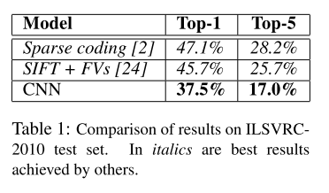
- 2010年，也就是ILSVRC竞赛举办的第一年，作者就参加了
- 这是测试集结果，ILSVRC-2010 测试集标签公开
- 表中第一行、第二行是其他人的方案取得的最好结果
  - 第一行：在不同特征上训练的稀疏编码模型，预测结果取平均
  - 第一行：在 Fisher Vector 上训练的两个分类器，预测结果取平均，其中Fisher Vector由两种类型的稠密采样特征计算得到
  - 这些方案不是端到端的
- 表中第三行，当时他们的方案就是CNN
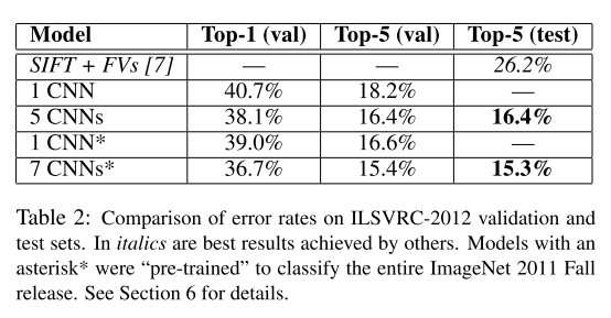
- ILSVRC-2012 测试集标签不公开，所以从训练数据划出了一部分验证集
- 第一行其他人的方案，ILSVRC-2012 第二名
- 第二行：本文描述的CNN架构
- 第三行：5个CNN模型，预测结果取平均
- 第四行（*表示使用了预训练）：1个CNN + extra sixth convolutional layer over the last pooling layer
  - 在整个 ImageNet 2011 Fall Release(15M images, 22K categories)上预训练，然后 fine-tuning on ILSVRC-2012
- 第五行（*表示使用了预训练）：2个CNN + 第三行的5个CNN
  - 前2个CNN在整个 ImageNet 2011 Fall Release(15M images, 22K categories)上预训练，然后 fine-tuning on ILSVRC-2012
使用不同的激活函数，神经网络预测错误率下降速度对比
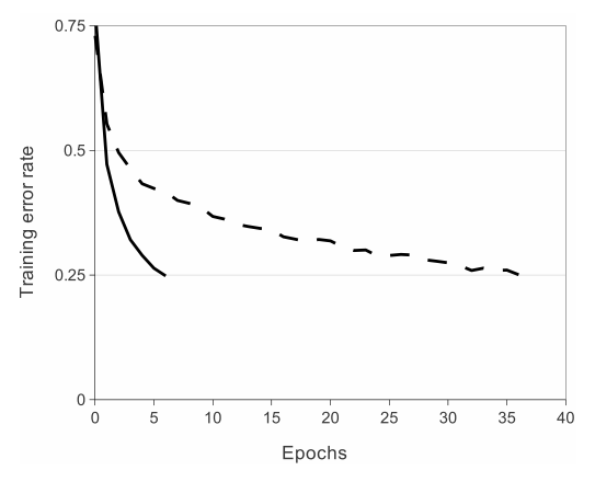
- 一个4层的卷积神经网络，在CiFAR-10上训练，虚线是使用 tanh 激活函数，实线是用 ReLU 激活函数
- 使用 ReLU 激活函数比 tanh 快6倍，后一个激活函数计算量大
模型学到了什么？
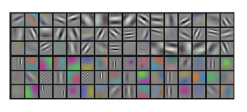
- 上图每行16个grid，共6行，每个grid代表一个kernel
- 前三行的结果是 conv1 在第一块GPU 48 个卷积核的可视化效果，color-agnostic
- 后三行的结果是 conv1 在第二块GPU 48 个卷积核的可视化效果，color-specific
- 作者说这种特殊现象在每次运行期间都会发生，与特定的随机初始化权重方法无关
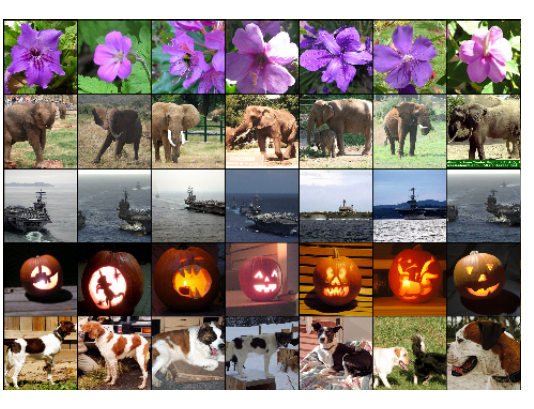
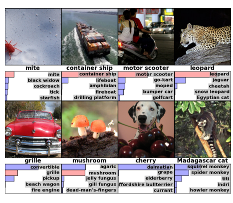
- 上图第1列的图片来自测试集；剩余的6列来自训练集，并且有如下关系
  - 这些测试集、训练集的图片，经过AlexNet 最后一个 hidden layer 产生的特征向量，Euclidean distance最小

PyTorch 实现

定义 AlexNet 网络结构

 import torch
 import torch.nn as nn

 class AlexNet(nn.Module):
     def __init__(self, num_classes=1000):
         super(AlexNet, self).__init__()
         self.features = nn.Sequential(
             nn.Conv2d(3, 96, kernel_size=11, stride=4, padding=2),
             nn.ReLU(inplace=True),
             nn.MaxPool2d(kernel_size=3, stride=2),
             nn.Conv2d(96, 256, kernel_size=5, padding=2),
             nn.ReLU(inplace=True),
             nn.MaxPool2d(kernel_size=3, stride=2),
             nn.Conv2d(256, 384, kernel_size=3, padding=1),
             nn.ReLU(inplace=True),
             nn.Conv2d(384, 384, kernel_size=3, padding=1),
             nn.ReLU(inplace=True),
             nn.Conv2d(384, 256, kernel_size=3, padding=1),
             nn.ReLU(inplace=True),
             nn.MaxPool2d(kernel_size=3, stride=2),
         )
         self.classifier = nn.Sequential(
             nn.Dropout(),
             nn.Linear(256 * 6 * 6, 4096),
             nn.ReLU(inplace=True),
             nn.Dropout(),
             nn.Linear(4096, 4096),
             nn.ReLU(inplace=True),
             nn.Linear(4096, num_classes),
         )

     def forward(self, x):
         x = self.features(x)
         x = torch.flatten(x, 1)
         x = self.classifier(x)
         return x

 def alexnet(pretrained=False, progress=True, **kwargs):
     """
     Args:
         pretrained (bool): If True, returns a model pre-trained
                            on ImageNet
         progress (bool): If True, displays a progress bar of the
                          download to stderr
     """
     model = AlexNet(**kwargs)
     if pretrained:
         state_dict = load_state_dict_from_url(model_urls['alexnet'],
                                               progress=progress)
         model.load_state_dict(state_dict)
     return model

定义一些对图片的操作，在加载数据时应用这些操作

 import torchvision.transforms as transforms

 transform = transforms.Compose([
     transforms.Resize(256),
     transforms.CenterCrop(224),
     transforms.ToTensor(),
     transforms.Normalize(mean=[0.485, 0.456, 0.406],
                          std=[0.229, 0.224, 0.225]),
 ])

准备训练图片、测试图片、标签数据

 import torchvision

 train_data = torchvision.datasets.ImageNet(
     root='./data', 
     train=True, 
     download=True, 
     transform=transform
 )
 trainloader = torch.utils.data.DataLoader(
     train_data, 
     batch_size=4, 
     shuffle=True, 
     num_workers=2
 )

 test_data = torchvision.datasets.ImageNet(
     root='./data', 
     train=False, 
     download=True, 
     transform=transform)
 testloader = torch.utils.data.DataLoader(
     test_data, 
     batch_size=4, 
     shuffle=False, 
     num_workers=2
 )

 with open('image_classes.txt') as f:
 classes = [line.strip() for line in f.readlines()]

【可选】对数据进行可视化

 import matplotlib.pyplot as plt
 import numpy as np

 # function to show some random images
 def imshow(img):
     img = img / 2 + 0.5     # unnormalize
     npimg = img.numpy()
     plt.imshow(np.transpose(npimg, (1, 2, 0)))
     plt.show()

 # get some random training images
 dataiter = iter(trainloader)
 images, labels = dataiter.next()

 # show images
 imshow(torchvision.utils.make_grid(images))
 # print labels
 print(' '.join('%5s' % classes[labels[j]] for j in range(4)))

准备AlexNet模型，并查看模型结构

 model = alexnet()

 # check model architecture or description
 model.eval()

【可选】对某些数据集，需要改变物体类别数目、全连接层输入/输出维度，

 # updating the second classifier
 model.classifier[4] = nn.Linear(4096,1024)

 # updating the third and the last classifier 
 # that is the output layer of the network.
 model.classifier[6] = nn.Linear(1024,10)

设置使用 GPU / CPU 设备

 # initializing a device 
 device = torch.device("cuda:0" if torch.cuda.is_available() else "cpu")

 print(device)

 # move model to the specified device
 model.to(device)

定义损失函数、优化器，开始训练 AlexNet

 import torch.optim as optim

 # set loss function
 criterion = nn.CrossEntropyLoss()

 # set optimizer
 optimizer = optim.SGD(model.parameters(), lr=0.001, momentum=0.9)

 # loop over the dataset multiple times
 epochs = 90

 for epoch in range(epochs):
     running_loss = 0.0
     for i, data in enumerate(trainloader, 0):
         # get the inputs; data is a list of [inputs, labels]
         inputs, labels = data[0].to(device), data[1].to(device)

         # zero the parameter gradients
         optimizer.zero_grad()

         # forward + backward + optimize
         output = model(inputs)
         loss = criterion(output, labels)
         loss.backward()
         optimizer.step()

         # print statistics
         running_loss += loss.item()
         if i % 2000 == 1999:    # print every 2000 mini-batches
             print('[%d, %5d] loss: %.3f' %
                 (epoch + 1, i + 1, running_loss / 2000))
             running_loss = 0.0

 print('Finished Training of AlexNet')

测试刚刚训练的 AlexNet

 # testing Accuracy
 correct = 0
 total = 0
 with torch.no_grad():
     for data in testloader:
         # move input images and labels to specified device
         images, labels = data[0].to(device), data[1].to(device)
         outputs = model(images)
         _, predicted = torch.max(outputs.data, 1)
         total += labels.size(0)
         correct += (predicted == labels).sum().item()

 print('Accuracy of the network on the 10000 test images: \
        %d %%' % (100 * correct / total))

AlexNet

简介

相关工作

模型结构

一些实现细节

实验

PyTorch 实现

Leave a Comment